Optical-Inertial Sensor Fusion

Optical position tracking and inertial orientation tracking are well established measurement methods. Each of these methods has its specific advantages and disadvantages. In this post we show an opto-inertial sensor fusion algorithm that joins the capabilities of both to create a capable system for position and orientation tracking.

How It Works

The reliability of position and orientation data provided by an optical tracking system (outside-in or inside-out) can for some applications be compromised by occlusions and slow system reaction times. In such cases it makes sense to combine optical tracking data with information from an inertial measurement unit located on the device. Our optical-intertial sensor fusion algorithm implements this functionality for integration with an existing tracking system or for the development of a novel system for a specific application case.

The graphs below show two examples of how the signal from an optical positioning system can be improved using inertial measurements. Slow camera framerates or occasional drop-outs are compensated by information from the integrated inertial measurement unit, improving the overall tracking performance.

Combination of Several Optical Trackers

For a demonstration, we combined three NEXONAR IR trackers and an LPMS-B2 IMU, mounted together as a hand controller. The system allows position and orientation tracking of the controller with high reliability and accuracy. It combines the strong aspects of outside-in IR tracking with inertial tracking, improving the system’s reaction time and robustness against occlusions.

Optical-Inertial Tracking in VR

The tracking of virtual reality (VR) headsets is one important area of application for this method. To keep the user immersed in a virtual environment, high quality head tracking is essential. Using opto-inertial tracking technology, outside-in tracking as well as inside-out camera-only tracking can be significantly improved.

Robot Operating System and LP-Research IMUs? Simple!

NOTE: We have released a new version of our ROS / ROS 2 driver, please refer to this post.


Introduction

Robot Operating System (ROS) is a tool commonly used in the robotics community to pass data between various subsystems of a robot setup. We at LP-Research are also using it in various projects, and it is actually very familiar to our founders from the time of their PhDs. Inertial Measurement Units are not only a standard tool in robotics, the modern MEMS devices that we are using in our LPMS product line are actually the result of robotics research. So it seemed kind of odd that an important application case for our IMUs was not covered by our LpSensor software: namely, we didn’t provide a ROS driver.  We are very happy to tell you that such a driver exists, and we are happy that we don’t have to write it ourselves: the Larics laboratory at the University of Zagreb are avid users of both ROS and our LPMS-U2 sensors. So, naturally, they developed a ROS driver which they provide on their github site.  Recently, I had a chance to play with it, and the purpose of this blog post is to share my experiences with you, in order to get you started with ROS and LPMS sensors on your Ubuntu Linux system.

Installing the LpSensor Library

Please check our download page for the latest version of the library, at the time of this writing it is 1.3.5. I downloaded it, and then followed these steps to unpack and install it:

I also installed libbluettoth-dev, because without Bluetooth support, my LPMS-B2 would be fairly useless.

Setting up ROS and a catkin Work Space

If you don’t already have a working ROS installation, follow the ROS Installation Instructions to get started. If you already have a catkin work space you can of course skip this step, and substitute your own in what follows.  The work space is created as follows, note that you run catkin_init_workspace inside the src sub-directory of your work space.

Downloading and Compiling the ROS Driver for LPMS IMUs

We can now download the driver sources from github. It optionally makes use of and additional ROS module by the Larics laboratory which synchronizes time stamps between ROS and the IMU data stream.  Therefore, we have to clone two git repositories to obtain all prerequisites for building the driver.

That’s it, we are now ready to run catkin_make to get everything compiled and ready.  Building was as simple as running catkin_make, but you should setup the ROS environment before that.  If you haven’t, here’s how to do that:

This should go smoothly. Time for a test.

Not as Cool as LpmsControl, but Very Cool!

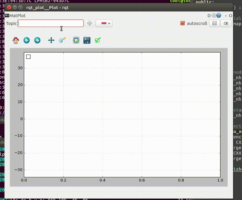
Now that we are set up, we can harness all of the power and flexibility of ROS. I’ll simply show you how to visualize the data using standard ROS tools without any further programming.  You will need two virtual terminals.  In the first start roscore, if you don’t have it running yet.  In the second, we start rqt_plot in order to see the data from our IMU, and the lpms_imu_node which provides it.  In the box you can see the command I use to connect to my IMU. You will have to replace the _sensor_model and _port strings with the values corresponding to your device.  Maybe it’s worth pointing out that the second parameter is called _port, because for a USB device it would correspond to its virtual serial port (typically /dev/ttyUSB0).

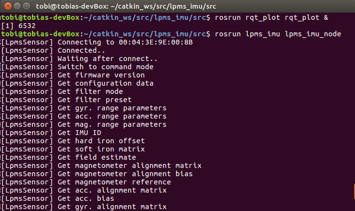
Once you enter these commands, you will then see the familiar startup messages of LpSensor as in the screenshot below. As you can see the driver connected to my LPMS-B2 IMU right away. If you cannot connect, maybe Bluetooth is turned off or you didn’t enter the information needed to connect to your IMU.  Once you have verified the parameters, you can store them in your launch file or adapt the source code accordingly.

Screenshot starting LPMS ROS node

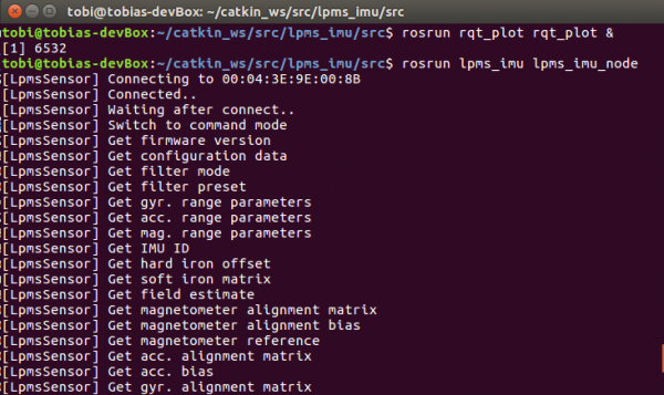
Screenshot of starting the LPMS ROS node

The lpms_imu_node uses the standard IMU and magnetic field message types provided by ROS, and it publishes them on the imu topic.  That’s all we need to actually visualize the data in realtime.  Below you can see how easy that is in rqt_plot. Not as cool as LpmsControl, but still fairly cool. Can you guess how I moved my IMU?

animation of how to display LPMS sensor data in ROS

Please get in touch with us, if you have any questions, or if you found this useful for your own projects.

Update: Martin Günther from the German Research Center for Artificial Intelligence was kind enough to teach me how to pass ROS parameters on the command line.  I’ve updated the post accordingly.

Race Car Stabilization – Team StarCraft at the Formula Student Germany

Team Starcraft's race car

Team StarCraft’s race car

From August 8-14 Team StarCraft of German Technische Universität Ilmenau participated at the Formula Student Germany – International Design Competition. Among many other teams from around the world they took on various challenges including acceleration and endurance races. Sensors such as the IMU (inertial measurement unit) from LP-RESEARCH offered valuable data about air pressure, vertical acceleration and magnetic field strength, which the racing team needed to regulate their traction control in order to perform well. The students used our LPMS-CU to control the car’s Torque Vectoring and the Anti-slip Regulation (ASR).
For next year’s race they will be back with an even more refined car!

Control of Autonomous Drone iHSMD

iHMSD is an autonomous, high-altitude glider developed by the European Space Agency (ESA) and Swiss companies Meteolabor, CSEM and Team SmartFish. Purpose of the project was to develop a light-weight, cost-efficient vehicle that can accurately navigate in extreme heights. The glider was towed up to 32km above ground level by weather balloons and then released to follow several waypoints and return safely to ground.

iHMSD test flight

Figure 1 – iHMSD flight test in good weather conditions over Switzerland.

High altitude flight tests were done at ESRANGE, Kiruna, Sweden. During the Swedish missions, the 1‑kg glider navigated through winds of almost 200 km/h, equivalent to a hurricane of category 4. Nonetheless, several very successful missions were flown, with the iHMSD vehicle reaching maximum speeds of almost Mach 0.9 and gathering many hours of flight data and video footage.

The iHMSD test flights reached a maximum altitude of 32000 meters and supersonic speed (1070 km/h).

LPMS-CURS was used by the team to measure exposure of the vehicle to strong accelerations and rotations. A control algorithm was implemented to adjust the steering of the glider to guarantee the accurate navigation of the prescribed waypoints.

Figure 2 – Together with other control electronics LPMS-CURS was installed in iHMSD to measure and adjust the flight stability of the glider.

Documentation about this fantastic project was provided to us by CSEM in Switzerland. Thank you!

The team around iHSMD created a video that documents the development process and the experiments:

LPMS-CU in ETH Zuerich Formula Student Race Car Flüela

Formula Student Electric Race Car Flüela

Flüela is the fourth four-wheel-driven Formula Student electric race car from the academic motorsports club Zurich. Four self-developed wheel-hub motors with a peak power of 37 kW while weighing only 3.25 kg enable an acceleration from 0-100 km/h in only 1.9s. A lithium polymer accumulator with a capacity of 6.46kWh supplies the car with the needed energy. The self-built carbon fibre monocoque enables a total weight of only 173 kg. Furthermore, the car uses adaptive dampers, which are unique in Formula Student, to adjust the damping forces dynamically to the driving situation. Miscellaneous control algorithms like torque vectoring and traction control ensure the car to deliver its maximum performance at every time of the race.

With Flüela the academic motorsports club Zurich was able to finish two out of four events overall on first place, as well as a second place in Formula Student Germany. The AMZ was able to defend its first place on the world ranking of the Formula Student Electric, and to finish the third year in a row as world champion.

Figure 1 – Flüela in Skidpad at Formula Student Spain.

Implementation of LPMS-CU in Flüela

The IMU was implemented in the back of the car. The major decision point of the placement was to set it near to the centre of the gravity of the whole car, including a driver. It was placed under the driver’s seat, next to the accumulator box. Tests were done to see if the high currents next to the accumulator box had any influence on the signal quality coming from the IMU. There were no electromagnetic influences detected. But we were not able to see if the high currents at full torque on the motors or while full recuperation (~200A) and their induced magnetic fields had any negative influence on the measured signals from the IMU. The problem there was that while driving at high speeds, there are further disturbances coming from vibrations of the car.

Figure 2 – Installation of LPMS-CU.

Applications of Sensor Data
Vehicle Dynamics Control

The three for our application most important signals coming from the LPMS-CU IMU were the accelerations in x (longitudinal, direction of travel) and y (lateral, direction of the front and rear axle) direction, as well as the rotation rate around the z-axis (vertical direction), further called the yaw rate of the car.

These signals were important inputs for our vehicle dynamics control system. The signal from the IMU has important influences in both, torque vectoring and traction control, as well as several smaller control algorithms used to maximise the performance of the race car.

Furthermore, some points are described, where the signals from the IMU were used in the vehicle dynamics control system:

1. Weight transfer calculation: One important thing to know for calculating the maximum torque which can be used by the tire is the force in z direction at every tire. To calculate this value, we use the accelerations in x and y direction to determine the chassis movement, and to calculate the forces on every single tire.

2. Mu estimator: We are able to adjust the used friction coefficient to calculate the possible deliverable forces of the tires. Depending on the track and the outer conditions, the friction coefficient (mu) is increased or decreased. For this calculations we need the absolute force which is acting on the car in x-direction, which can be calculated by the longitudinal acceleration and the mass of the car.

3. Torque vectoring: The yaw rate is the most important value for our torque vectoring system. By using a simplified vehicle model, we calculate the optimal yaw rate for every corner at every time. This calculated value is then compared to the actual measured value by the IMU, and an occurring error is corrected by an adjusted torque distribution on every wheel.

Data Analysis

Furthermore, the data coming from the IMU was very important for data analysis. One example of the usage of the signals is the G-G-Plot, a classical way to look at the performance of the system car and driver.

Figure 3 – G-G-Plot of the Autocross event in Austria.

We also used the data from the IMU and the Absolute Speed Sensor (optical measurement of the speed of the car) to approximate the course of the track. These track plots were used to display at which point of the track the accelerations on the car were at a maximum.

In Figure 4 we are able to see at which parts of the track the potential of the car is used, and where higher total accelerations would be possible. In the red parts, the cars potential is used at a maximum, in the blue parts the car-driver system could have performed better.

Figure 4 – Track plot Autocross Austria.

Thank you to Formula Student Team Zurich for the detailed report. For further information on the team, please have a look at their website.

1 2 3 4 5